Example-19: Layout
[1]:
# In this example graphical representation of (planar) layout if illustrated
# Layout data can be generated to draw layout in 1D, 2D and 3D along with other curves (given on sliced lattice)
# To avoid explicit dependencies on graphical libraries (matplotlib and plotly), results are returned as dictionaries
[2]:
# Import
import matplotlib
from matplotlib import pyplot as plt
from matplotlib.patches import Rectangle
matplotlib.rcParams['text.usetex'] = True
from plotly import graph_objects
import torch
from twiss import twiss
from twiss import propagate
from twiss import wolski_to_cs
from model.library.drift import Drift
from model.library.quadrupole import Quadrupole
from model.library.sextupole import Sextupole
from model.library.dipole import Dipole
from model.library.bpm import BPM
from model.library.line import Line
from model.command.layout import Layout
[3]:
# Define simple FODO based lattice
QF = Quadrupole('QF', 0.5, +0.20)
QD = Quadrupole('QD', 0.5, -0.19)
SF = Sextupole('SF', 0.25)
SD = Sextupole('SD', 0.25)
DR = Drift('DR', 0.25)
BM = Dipole('BM', 3.50, torch.pi/4.0)
BA = BPM('BA', direction='inverse')
BB = BPM('BB', direction='forward')
FODO = Line('FODO',
[BA, QF, DR, SF, DR, BM, DR, SD, DR, QD, QD, DR, SD, DR, BM, DR, SF, DR, QF, BB],
propagate=True,
dp=0.0,
exact=False,
output=True,
matrix = True)
RING = Line('RING',
4*[FODO],
propagate=True,
dp=0.0,
exact=False,
output=True,
matrix = True)
[4]:
# Perform lattice slicing
# Note, one step is used for zero length elements
RING.ns = 0.05
print(RING.ns)
{'BA': 1, 'QF': 10, 'DR': 5, 'SF': 5, 'BM': 70, 'SD': 5, 'QD': 10, 'BB': 1}
[5]:
# Compute transport matrices along closed orbit
state = torch.tensor([0.0, 0.0, 0.0, 0.0], dtype=torch.float64)
print(torch.func.jacrev(RING)(state))
print()
total, *ms = RING.container_matrix
for m in ms:
total = m @ total
print(total)
print()
tensor([[ -0.3382, -17.5116, 0.0000, 0.0000],
[ 0.0506, -0.3382, 0.0000, 0.0000],
[ 0.0000, 0.0000, -0.2976, -6.0422],
[ 0.0000, 0.0000, 0.1508, -0.2976]], dtype=torch.float64)
tensor([[ -0.3382, -17.5116, 0.0000, 0.0000],
[ 0.0506, -0.3382, 0.0000, 0.0000],
[ 0.0000, 0.0000, -0.2976, -6.0422],
[ 0.0000, 0.0000, 0.1508, -0.2976]], dtype=torch.float64)
[6]:
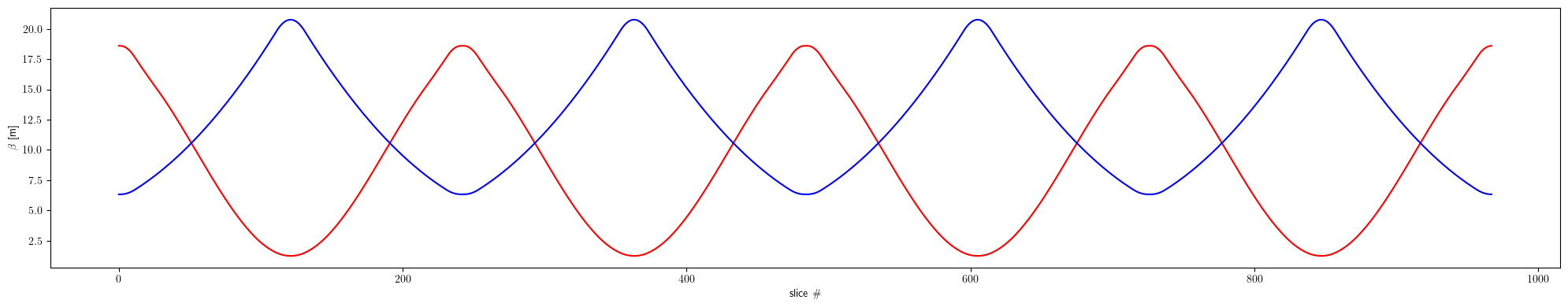
# Compute twiss parameters at slices (entrance of each slice)
# Compute twiss from one-turn matrix at starting location
(nux, nuy), _, w = twiss(total)
# Print fractional tunes
print(f'{nux.item(), nuy.item()}')
# Propagate twiss parametes
ws = [w]
*ms, _ = RING.container_matrix
for m in ms:
w = propagate(w, m)
ws.append(w)
ws = torch.stack(ws)
# Convert to CS and plot beta functions
_, bx, _, by = torch.vmap(wolski_to_cs)(ws).T
plt.figure(figsize=(20, 4))
plt.plot(bx.cpu().numpy(), color='red', label=r'$\beta_x$')
plt.plot(by.cpu().numpy(), color='blue', label=r'$\beta_y$')
plt.xlabel(r'slice \#')
plt.ylabel(r'$\beta$ [m]')
plt.tight_layout()
plt.show()
(0.6950865039372625, 0.7018998427861426)
[7]:
# Generate several trajectories on slice (turn off matrix computation)
RING.matrix = False
state = torch.tensor([+0.01, 0.0, -0.01, 0.0], dtype=torch.float64)
orbit = []
for _ in range(16):
state = RING(state)
orbit.append(RING.container_output.clone())
orbit = torch.stack(orbit)
orbit.shape
[7]:
torch.Size([16, 968, 4])
[8]:
# Set layout
layout = Layout(RING)
[9]:
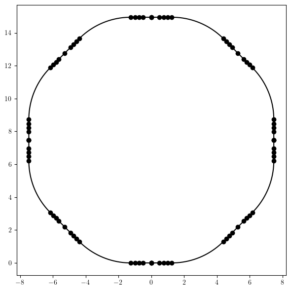
# Reference orbit (lines and arcs)
# With step = None, returns globals coordinates for elements entrance faces (if the last entry is dropped)
x_entrance, y_entrance, *_ = layout.orbit(flat=False, step=None)
# Step size can be passed to generate smooth closed orbit curve
# Slicing is performed only in arc sections
x, y, *_ = layout.orbit(flat=False, step=0.01)
plt.figure(figsize=(6, 6))
plt.scatter(x_entrance.cpu().numpy(), y_entrance.cpu().numpy(), marker='o', color='black')
plt.plot(x.cpu().numpy(), y.cpu().numpy(), color='black')
plt.tight_layout()
plt.show()
# Note, rotation is anti-clockwise
[10]:
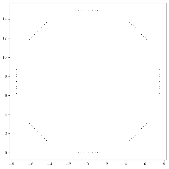
# Information about each element
# (name, kind, length, angle)
names, kinds, lengths, angles = zip(*layout.line.layout())
# Element locations in global frame can be computed using orbit method
x, y, *_ = layout.orbit(step=None, flag=False, lengths=lengths, angles=angles)
plt.figure(figsize=(6, 6))
plt.errorbar(x.cpu().numpy(), y.cpu().numpy(), fmt=' ', ms=1, marker='x', color='black')
plt.tight_layout()
plt.show()
[11]:
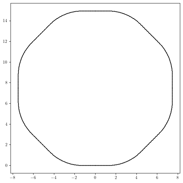
# In sliced lattice each element is splitted into one or more slices
# Information about each slice
# (name, kind, length, angle, point)
# Here point gives element entrance face location in global coordinate system
names, kinds, lengths, angles, points = layout.slicing_table()
x, y, *_ = points.T
plt.figure(figsize=(6, 6))
plt.errorbar(x.cpu().numpy(), y.cpu().numpy(), fmt=' ', ms=1, marker='x', color='black')
plt.tight_layout()
plt.show()
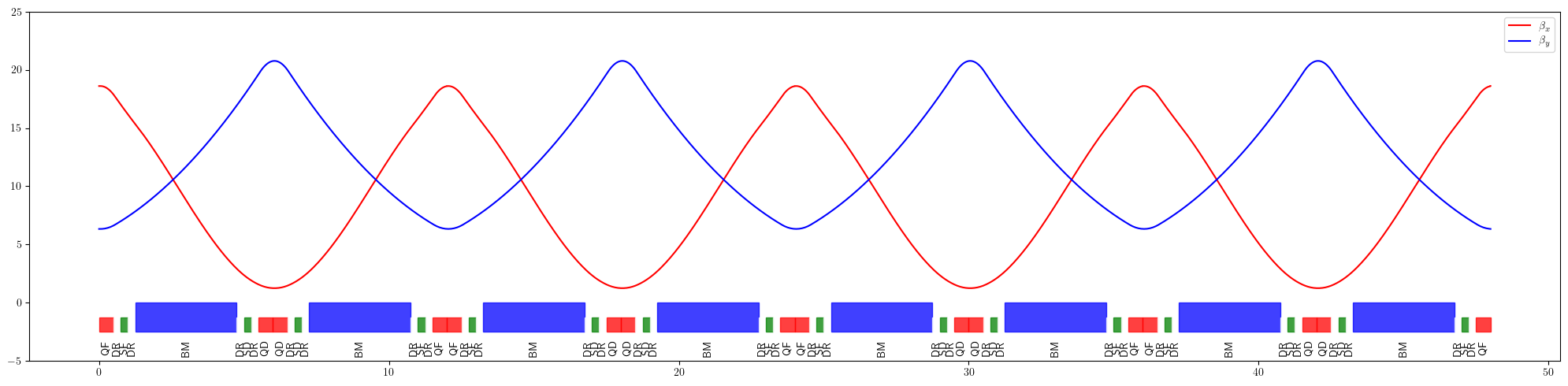
[12]:
# 1D profile (rectangles)
_, _, lengths, *_ = layout.slicing_table()
rectangles, labels = layout.profile_1d(scale=5.0,
shift=-2.5,
text=True,
delta=-4.0,
rotation=90,
exclude=['BPM'])
plt.figure(figsize=(20, 5))
plt.plot(lengths.cumsum(-1).cpu().numpy(), bx.cpu().numpy(), color='red', label=r'$\beta_x$')
plt.plot(lengths.cumsum(-1).cpu().numpy(), by.cpu().numpy(), color='blue', label=r'$\beta_y$')
plt.legend()
for rectangle in rectangles:
plt.gca().add_patch(Rectangle(**rectangle))
for label in labels:
plt.text(**label)
plt.ylim(-5.0, 25.0)
plt.tight_layout()
plt.show()
# Default colors and other parametes are defined in config attribute (layout class variable)
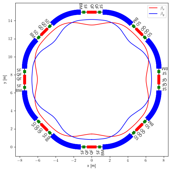
[13]:
# 2D profile and data transformation
# Using angles and global positions, data on slices can be transformed
# In general, data scaling should be adjusted to present transformed data in appealing way\
# Transform data
*_, angles, points = layout.slicing_table()
angles = angles.cumsum(-1)
bx_x = torch.zeros_like(bx)
bx_y = +(0.05*bx + 0.5)
bx_z = torch.zeros_like(bx)
bx_points = torch.stack([bx_x, bx_y, bx_z]).T
bx_x, bx_y, bx_z = torch.vmap(layout.transform)(bx_points, points, angles).T
by_x = torch.zeros_like(by)
by_y = +(0.05*by + 0.5)
by_z = torch.zeros_like(by)
by_points = torch.stack([by_x, by_y, by_z]).T
by_x, by_y, by_z = torch.vmap(layout.transform)(by_points, points, angles).T
# Generate reference orbit
x, y, _ = layout.orbit(flat=False, step=0.01, start=(0, 0))
# Generate layout
blocks, labels = layout.profile_2d(start=(0, 0),
delta=-0.6,
linewidth=1.5,
exclude=['Drift', 'BPM'])
# Plot
plt.figure(figsize=(6, 6))
plt.plot(x, y, color='black')
plt.plot(bx_x, bx_y, color='red', label=r'$\beta_x$')
plt.plot(by_x, by_y, color='blue', label=r'$\beta_y$')
for block in blocks:
plt.errorbar(**block)
for label in labels:
plt.text(**label)
plt.legend()
plt.xlabel(r'x [m]')
plt.ylabel(r'y [m]')
plt.tight_layout()
plt.show()
[14]:
# 3D profile and data transformation
names, kinds, lengths, angles, points = layout.slicing_table()
angles = angles.cumsum(-1)
# Transform orbits
scale = 50.0
qx, _, qy, _ = orbit.swapaxes(0, 1).swapaxes(0, -1)
q_x = scale*torch.zeros_like(qx)
q_y = scale*qx
q_z = scale*qy
q_points = torch.stack([q_x, q_y, q_z]).swapaxes(0, -1)
q_x, q_y, q_z = torch.vmap(layout.transform)(q_points, points, angles).swapaxes(0, -1)
# Select data at BPMs
q_x_bpm = []
q_y_bpm = []
q_z_bpm = []
for kind, qx, qy, qz in zip(kinds, q_x.T, q_y.T, q_z.T):
if kind == 'BPM':
q_x_bpm.append(qx)
q_y_bpm.append(qy)
q_z_bpm.append(qz)
q_x_bpm = torch.stack(q_x_bpm)
q_y_bpm = torch.stack(q_y_bpm)
q_z_bpm = torch.stack(q_z_bpm)
# Generate reference orbit
x, y, z = layout.orbit(flat=False, step=0.01, start=(0, 0))
# Generate layout (can be saved as html with write_html method)
blocks = layout.profile_3d(scale=1.75)
# Plot
figure = graph_objects.Figure(
data=[
graph_objects.Scatter3d(
x=x.numpy(),
y=y.numpy(),
z=z.numpy(),
mode='lines',
name='Orbit',
line=dict(color='black',width=2.0,dash='solid'),
opacity=0.75,
showlegend=True
),
graph_objects.Scatter3d(
x=q_x.flatten().numpy(),
y=q_y.flatten().numpy(),
z=q_z.flatten().numpy(),
mode='lines',
name='Trajectory',
line=dict(color='black',width=1.0,dash='solid'),
opacity=0.50,
showlegend=True
),
graph_objects.Scatter3d(
x=q_x_bpm.flatten().numpy(),
y=q_y_bpm.flatten().numpy(),
z=q_z_bpm.flatten().numpy(),
mode='markers',
name='Projection',
marker=dict(color='red',size=1.5),
opacity=0.50,
showlegend=True
),
*[graph_objects.Mesh3d(block) for block in blocks]
]
)
figure.update_layout(
scene=dict(
xaxis=dict(visible=False, range=[-20,20]),
yaxis=dict(visible=False, range=[-20,20]),
zaxis=dict(visible=False, range=[-5,5]),
aspectratio=dict(x=1, y=1, z=1/4),
annotations=[]
),
margin=dict(l=0, r=0, t=0, b=0),
legend=dict(orientation='v', x=0., y=1., xanchor='left', yanchor='top'),
hoverlabel=dict(font_size=12, font_family="Rockwell", font_color='white'),
legend_groupclick='toggleitem'
)
figure.show()